
February 29, 2024 •Olivia Hebner
With contributions by Kathryn Cronquist, Thienthanh Trinh, Paige Hayward, Shannon Houser, and Nicole Schwartz
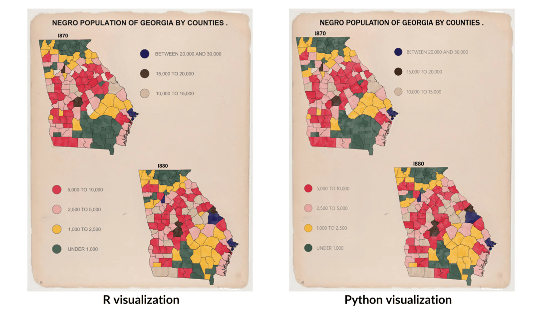
In celebration of Black History Month, a group of Summiteers participated in the 2024 Du Bois Visualization Challenge. This challenge was created by the Data Visualization Society to celebrate the data visualization legacy of W.E.B. Du Bois, a Black American civil rights activist, sociologist, and writer, by re-creating his visualizations from the 1900 Paris Exposition using modern tools. Our team ultimately decided to split into two groups to re-create Du Bois’s Plate 6 (original image below) using both R and Python.
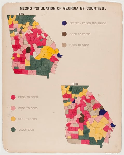
The data were provided by the Data Visualization Society in their GitHub repository. Both teams used the provided shapefile, which contains the geometry data as well as the total population range by county for 1870 and 1880. The teams transformed the coordinate reference system of the shapefile to a World Geodetic System 1984 (WGS84) projection. The WGS84 projection is the most widely used geodetic reference system and ensured the maps appeared straight (without the transformation, each map was tilted).
Additionally, both teams imported census tract data using pygris in Python or tigris in R. The census tract data were used to create a shading effect in each county. To perform the shading, the teams randomly assigned a number to each census tract. This number was used as the transparency indicator (alpha). For example, an alpha of 0 indicates complete transparency and an alpha of 1 indicates complete opacity. By plotting the county map and census tract map together, the teams were able to achieve the shading effect.
Team R utilized sf and tigris to import the data, tidyverse to clean the data, and ggplot2 and grid to create the visualization.
Team R began with ggplot2 to create the 1870 and 1880 maps. After converting the 1870 and 1880 variables to factors and assigning a color palette and corresponding list of labels, they plotted the counties by population range. They then added the layer of census tracts to apply the shading effect. The team used theme_void() to display an empty background to the map.
The Team used viewports from grid to define the space. Viewports define a rectangular space on the plot, and a programmer can then place objects within each viewport relative to its dimensions. They created a parent viewport encompassing the full graphic and four individual viewports to hold the plots and legend sections separately. They used Normalized Parent Coordinates as the units throughout. This required estimating the spacing of the titles, maps, and legend markers and text in relation to the viewport’s coordinate system.
Finally, Team R filled in the viewports with the various figures and text. They centered the title near the top of the parent viewport and placed the 1870 and 1880 maps in the upper left and lower right viewports, respectively. Because each map did not extend to the edges of the viewport, the team overlapped the viewports to reduce the blank space between the maps. They then defined the legend using grid.circle to define the location, radius, and color of the markers and grid.text for the associated text label in an upper right and a lower left viewport. The team tested various fonts, text color and size, and marker radius to approximate the original visualization.
Team Python utilized GeoPandas and pygris to import the data, NumPy and pandas to clean the data, and matplotlib to create the visualization.
The team began by defining the color palette associated with each legend item and assigned the color palette to the total population range variables. Next, they created a figure with four subplots (a 2 x 2 grid). This allows the programmer to manipulate the subplots individually. Using the census tract data, the team assigned the randomly translucent map (described above) to subplot 1 (upper left quadrant) and subplot 4 (bottom right quadrant). Subplot 1 showed the populations in 1870, whereas subplot 4 showed the populations in 1880. Using the county shapefile, the team plotted the county-level maps layered with the census tract maps.
A custom legend was created and displayed in subplot 2 (upper right quadrant) and subplot 3 (lower right quadrant). Three variables were displayed in subplot 2 and four variables were displayed in subplot 3 using a custom-made legend in matplotlib. The team manipulated line style, marker size, marker edge color, and marker edge width to mimic the original visualization. Finally, the team tested various fonts, text colors, and text sizes to approximate the original visualization.

If you’re interested in more details, you can view our code on Summit’s GitHub.