Heckman Selection Bias Correction: Further Explanation
Whenever funds are spent to accomplish some goal—such as increasing young people’s earnings by training them for good jobs—program evaluators may be called upon to determine whether those funds have been spent successfully. A basic program evaluation regression model would be
Y = k + mX + qS +ɛ1,
where Y represents post-training earnings, X represents earnings-relevant individual characteristics (such as years of education), S=1 if an eligible individual participates in training, S = 0 if an eligible individual does not participate in training, k, m, and q are coefficients to be estimated, and ɛ1 is an error term assumed uncorrelated with S or X and normally distributed around a zero mean.
There are two reasons why these assumptions about the error term might be untenable.
- Self-selection may make those whose earnings would be higher than average even without training more likely to participate in training;
- “Creaming” to make their efforts look more effective might make program operators more likely to recruit those whose earnings would be higher than average even without training.
The “Heckman selection bias correction” attempts to correct these possible error term ɛ1 problems by assuming that S is properly observed only if Z + ɛ2 > 0,
where Z is a variable not included in X and the correlation between ɛ1 and ɛ2 = r. Z thus is a variable that affects poor young people’s decisions to apply for a training program but does not affect earnings directly. One example of Z might be the presence of a caring adult mentor in a young person’s life. In practice, many statisticians simply let Z = X, although Heckman would say that doing so leaves the impact estimate “not identified”.
If the correlation between the two error terms ɛ1 and ɛ2 is r, then
Z > – ɛ2 is equivalent to
Z > -(r x ɛ1) = c
This correction removes from the comparison of participants and nonparticipants those who would not apply for the program and those who would not be recruited by the program.
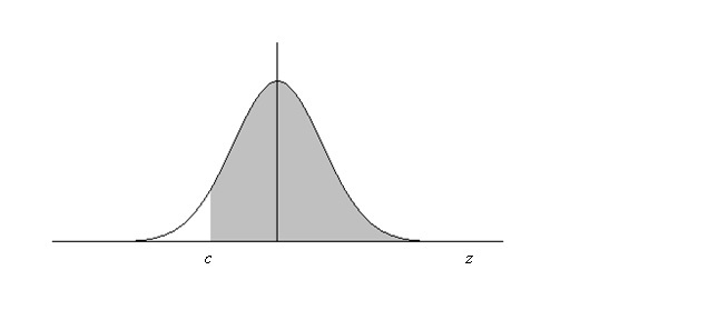
The figure below shows how the density of the error term ɛ1 is truncated by this selection correction. Rather than the full normal distribution, only the shaded portion is relevant to the selection-corrected comparison of participants and nonparticipants.
The expected value of a normally distributed error term is 0. But, what is the expected value of an error term in the shaded area? That is given by the inverse Mills ratio λ (named after statistician John P, Mills). Where phi is the normal density function and PHI is the cumulative normal distribution function,
λ (Z) = phi(c)/(1-PHI(c)). This quantity is a nonlinear function of Z that varies from one individual to another.
When r is nonzero, ordinary least-squares regression yields an estimate for the program impact d that is biased by amount λ(Z). So Heckman’s procedure adds λ(Z) to the original regression to remove the selection bias:
Y = a + dS + bX + w λ(Z) + ɛ1.
Coefficients a, d, b, and w now can be estimated by OLS without selection bias, assuming that the relationship between ɛ1 and ɛ2 is bivariate normal, and that a suitable selection variable Z has been used.


