Covariate Regression Adjustment: Further Explanation

Covariate Regression Adjustment: Further Explanation

Much of applied statistics focuses on comparing differences in policy-relevant average group outcomes.  These outcomes may include, for example–

• earnings,
• injury rates, or
• mortgage approval rates.

The groups that are compared also are policy-relevant; for example–

• veterans versus non-veterans;
• inspected workplaces versus uninspected workplaces; or
• black mortgage applicants versus white mortgage applicants.

To ensure that these comparisons are fair, and that outcome-influencing factors other than group membership are put aside, potential confounding covariates must be taken into account. Confounding covariates offer alternative explanations–rather than group membership–for group outcome differences.

For example, age often explains differences in earnings.  Because most people’s earnings grow with age except near retirement, any group of somewhat older workers tends to earn more than any group of somewhat younger workers. If group T happens to be older on average than group C, the age factor must be taken into account before group membership can be deemed responsible for all group earnings differences.

The table below shows the most common way statisticians take group differences in age (X) into account when comparing average earnings (Y) between group T and group C.  Assuming that the earnings trend is linear in age, and that the trend (slope) is the same for both groups, average earnings conditional on age can be represented by parallel lines, one for group T and one for group C.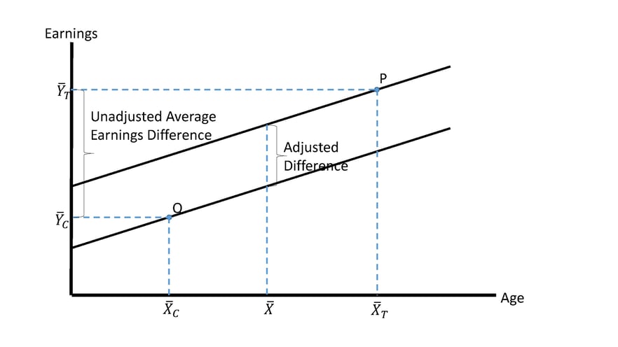

Notice that point P in the figure represents the average earnings and the average age for group T. Notice also that point Q represents the average earnings and the average age for group C.  The unadjusted difference in average earnings is denoted by the big bracket on the left.

Because Group T is older, it has an unfair earnings advantage over Group C. The age factor somehow must be taken into account.   This is most commonly accomplished using a form of linear regression called ANalysis of COVAriance (ANCOVA) or covariate “regression adjustment”.  When there is one covariate (X) and two groups, denoted by D=1 and D=0, the ANCOVA regression equation is simply

Y = a + bD + cX + ε,

where ɛ is a normally-distributed error term assumed uncorrelated with D or with X.  Minimizing the sum of the squares of distances between actual individual observations for Y and the values of Y predicted by the regression equation yields estimates of coefficients a, b, and c.  Coefficient estimate b is represented by the vertical distance between the two parallel lines in the figure.  Instead of comparing two actual groups with different average ages, the adjusted difference compares two counterfactual groups with identical average ages.

The next table overlays some refinements on Figure 1 to calculate precise values of adjusted means.

The grand mean of the age covariate across both groups must lie between the extremes of  and  . The ANCOVA procedure determines the mean outcomes each group would have achieved if their average ages had been equal to the grand mean age. Adjusting group T’s outcome slightly downward (downward arrow) and group C’s average slightly upward (upward arrow) makes the adjusted impact equal to the vertical difference between the two parallel lines. To determine how much each group’s average moves, simply multiply its horizontal distance from the grand mean age by the negative of the common age slope estimate:

If additional covariates are taken into account (such as years of education, school quality, prior work experience, gender, and race), the adjustment amount is the sum of several terms similar to the single term in the equation above.